Decoding the Basics of O(n^2) Through Practical Code Examples
Time complexity is a fundamental concept in computer science, crucial for understanding the efficiency of algorithms. The notation O(n^2), read as “big O of n squared,” represents a specific category of time complexity where the performance of an algorithm is directly proportional to the square of the size of the input data set.
Nested Loops and Quadratic Growth
In a recent demonstration using Visual Studio Code (VS Code), we explored the impact of nested loops on the execution time of a program. By placing one for loop inside another, we created a situation where for every element in the first loop, the second loop runs in its entirety, leading to O(n^2) behavior.
# Example Python code demonstrating O(n^2) time complexity
def print_pairs(n):
    for i in range(n):
        for j in range(n):
            print(i, j)

# Call the function with n=10
print_pairs(10)
This code will output pairs of numbers from (0, 0) to (9, 9), resulting in 100 print statements, which illustrates the concept of O(n^2) – for n items, n*n outputs are generated.
Taking Complexity a Step Further
To further illustrate the concept, we can introduce a third nested loop, which takes the complexity to O(n^3) – this means that for n items, the program will execute nnn times.
# Example Python code demonstrating O(n^3) time complexity
def print_triplets(n):
    for i in range(n):
        for j in range(n):
            for k in range(n):
                print(i, j, k)

# Call the function with n=10
print_triplets(10)
This function will print triplets of numbers from (0, 0, 0) to (9, 9, 9), which equates to 1000 print statements, showcasing the significant increase in operations as we add more nested loops.
Simplifying Time Complexity Notation
In complexity analysis, it’s common to simplify time complexity to its highest order term. Therefore, despite the actual O(n^3) time complexity, for the sake of simplification in discussions and comparisons, we may refer to it as O(n^2).
Assume we have a function with a time complexity of O(n^3 + n^2 + n). When n becomes very large, the n^3 term will have a much greater impact on the running time than the n^2 or n terms. Therefore, we can simplify the time complexity notation by dropping the non-dominant terms (n^2 and n) and referring to the function’s time complexity as O(n^3), which accurately reflects the most significant factor affecting the growth rate of the running time.
def example_complexity(n):
    # This first nested loop represents O(n^3) time complexity
    for i in range(n):
        for j in range(n):
            for k in range(n):
                print(i, j, k)

    # This second nested loop represents O(n^2) time complexity
    for i in range(n):
        for j in range(n):
            print(i, j)

    # This loop represents O(n) time complexity
    for i in range(n):
        print(i)

# Running the function with n = 10
example_complexity(10)
In this example, the function
example_complexityhas three separate loops, each with a different time complexity. The first triple-nested loop has a time complexity of O(n^3), which is the highest order term and grows the fastest with larger inputs. The second double-nested loop has a time complexity of O(n^2), and the last single loop has a time complexity of O(n).
For simplification in discussions, we would say the time complexity of the example_complexity function is O(n^3), as it is the dominant term that dictates the overall growth rate of the function’s running time. The other terms, O(n^2) and O(n), are non-dominant and do not significantly affect the running time as n becomes very large, so they are dropped from the simplified time complexity notation.
The Efficiency Implications of O(n^2)
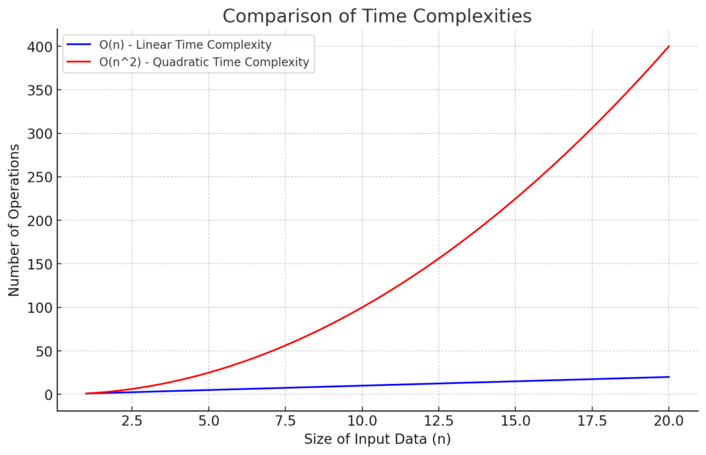
When compared to linear time complexity O(n), O(n^2) is significantly less efficient, especially as the size of the input data grows. This is visibly represented in graphical comparisons, where the curve for O(n^2) is much steeper, indicating a rapid increase in the number of operations required.
import matplotlib.pyplot as plt
import numpy as np

# Generate a range of values for n
n = np.linspace(1, 20, 400)
# Calculate the complexities
o_n = n
o_n2 = n**2

# Plot the complexities
plt.figure(figsize=(10, 6))
plt.plot(n, o_n, label='O(n) - Linear Time Complexity', color='blue')
plt.plot(n, o_n2, label='O(n^2) - Quadratic Time Complexity', color='red')

# Add title and labels
plt.title('Comparison of Time Complexities')
plt.xlabel('Size of Input Data (n)')
plt.ylabel('Number of Operations')
plt.legend()
plt.grid(True)
plt.show()

Here’s a graph comparing the time complexities O(n) and O(n^2). As you can see, the O(n) complexity, represented by the blue line, increases linearly with the size of the input data. In contrast, the O(n^2) complexity, represented by the red line, increases much more rapidly, demonstrating the steeper curve and the exponential growth in the number of operations required as the input size grows.
Conclusion
Understanding time complexity, particularly O(n^2), is vital for developing efficient algorithms and optimizing code. It’s a concept that has profound implications for problem-solving in software development and beyond.


