
Demystifying Big O: Starting with O(n)
Big O notation is a mathematical concept used in computer science to describe the performance or complexity of an algorithm. It’s a part of computational theory that allows developers and programmers to estimate how an algorithm scales as the size of the input data set increases. Today, we’ll be exploring O(n) complexity—often described as linear complexity, which is fundamental to understanding algorithm efficiency.
The Essence of O(n) Complexity
O(n) complexity, pronounced “Big O of n,” represents algorithms whose performance will grow linearly and in direct proportion to the size of the input data set. It’s one of the most common time complexities you’ll encounter, and it’s relatively easy to grasp. The “n” refers to the number of elements the algorithm must pass through to perform its function.
Illustrating O(n) with a Simple Code Example
To illustrate O(n) complexity, let’s consider a basic function in any programming language—printing each item in a list. Here’s a simple Python function that does just that:
def print_items(n):
    for i in range(n):
        print(i)

#Call the function with n=10
print_items(10)
This function, print_items, takes a single argument n and prints numbers from 0 to n-1. The number of print operations is directly proportional to n. If n is 10, it prints ten times. This direct correlation is why it’s considered O(n) complexity.
Visualizing O(n) Complexity
When plotted on a graph with n on the x-axis and the number of operations on the y-axis, O(n) complexity is represented by a straight line, indicating that the number of operations increases linearly with n. It is what is called proportional.
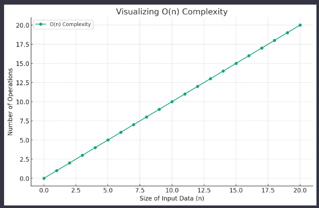
The graph visually represents O(n) complexity. As you can see, the relationship between the size of the input data (n) on the x-axis and the number of operations on the y-axis is linear, illustrating that the operations increase proportionally with n.
The Practicality of O(n) in Real-World Scenarios
O(n) complexity algorithms are quite common in real-world applications. For example, searching through a list to find an item, where the worst-case scenario is having to check every element, is an O(n) operation. It’s simple, straightforward, and often the first step in optimizing towards more efficient algorithms.
Conclusion
O(n) complexity serves as an excellent starting point for understanding algorithm performance. It is a crucial concept in software development, data analysis, and many other fields where algorithms play a significant role. As we move forward, we’ll compare O(n) to other types of complexities, deepening our understanding of algorithm efficiency.