Demystifying Constant Time Complexity: O(1) Explained
In the world of programming and algorithm optimization, understanding time complexity is crucial. Among the various complexity classes, O(1), also known as constant time complexity, stands out for its efficiency. Let’s dive into what O(1) means and how it applies to real-world programming scenarios.
The Concept of O(1) with an Example Function
Consider a simple function named add_items, which takes an integer n and returns the sum of n and n. Regardless of the size of n, the function performs just one operation – the addition. This is a classic example of an O(1) function. Here’s what the implementation might look like in Python:
def add_items(n):
    return n + n
The beauty of this function lies in its simplicity and predictability. Whether n is 1 or 1 million, add_items will always perform one operation, making it a constant time function.
Sample implementation:
def add_items(n):
    return n + n

# Example usage:
print(add_items(5))
print(add_items(1000000))
# Re-defining the O(1) function after execution state reset

def add_items(n):
    # This function performs a single operation regardless of the size of n, hence it's O(1)
    return n + n

# Example usage of the function
add_items_example_small = add_items(5)
add_items_example_large = add_items(1000000)

add_items_example_small, add_items_example_large
The function add_items is an example of an O(1) function in Python. It simply returns the sum of the input n plus itself, which is a single operation regardless of the size of n. Here’s how the function behaves with two different inputs:
- For
n = 5, the function returns10. - For
n = 1000000, the function returns2000000.
In both cases, the number of operations performed by the function remains constant, demonstrating the O(1) or constant time complexity.
Why O(1) Matters
The significance of O(1) is in its scalability. As your input size (n) increases, the time it takes to run your operation stays the same. This is unlike other time complexities where the number of operations increases with the size of the input. O(1) represents the ideal scenario in algorithm design – an operation that does not become slower as the dataset grows.
Graphical Representation of O(1)
import matplotlib.pyplot as plt
import numpy as np

# Generating a range of input sizes
input_sizes = np.arange(1, 10001, 500)

# Since the time complexity is O(1), the time taken is constant, let's assume it's 1 unit of time
time_taken = np.ones_like(input_sizes)

# Plotting the graph
plt.figure(figsize=(10, 6))
plt.plot(input_sizes, time_taken, label='O(1) Complexity', color='blue', linewidth=2)
plt.ylim(0.8, 1.2)  # Keep the y-axis tight to show the flat line more clearly
plt.title('Graph of O(1) Time Complexity')
plt.xlabel('Input Size (n)')
plt.ylabel('Time Taken (arbitrary units)')
plt.legend()
plt.grid(True)
plt.show()
If we were to graph the performance of an O(1) function, it would appear as a flat line, indicating that the time taken remains unchanged regardless of input size. This constant behavior is why O(1) is the golden standard in algorithm optimization.
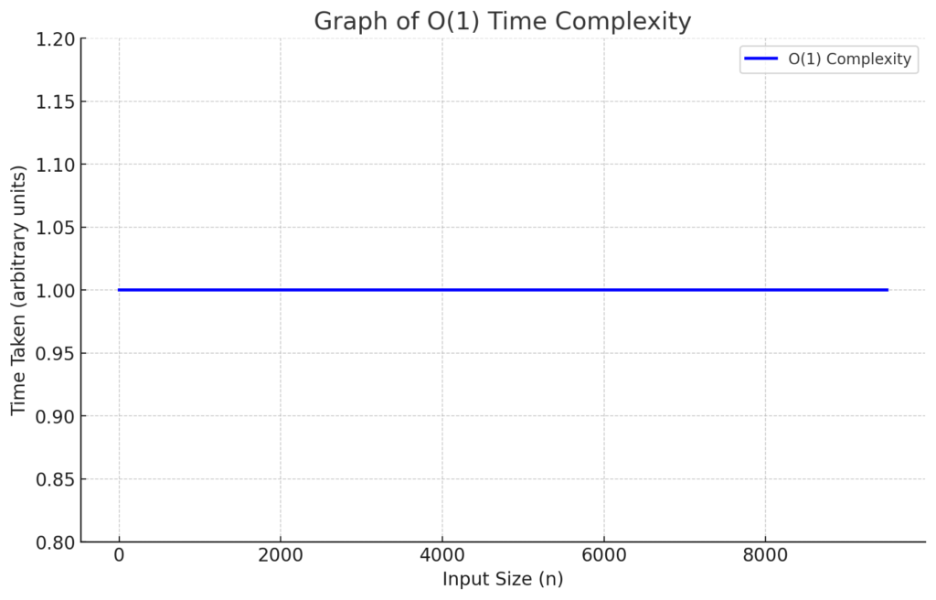
Here is the graph depicting the performance of an O(1) function. As shown, the time taken remains constant regardless of the input size, illustrated by the flat line across the graph. This constant behavior exemplifies why O(1) complexity is considered optimal in algorithm design
Optimization and Efficiency
The quest in programming is to achieve O(1) whenever possible. It represents the pinnacle of efficiency and is particularly relevant in high-performance computing where response time is critical.
Conclusion
In summary, O(1) complexity is a key concept in computer science that denotes operations that run in constant time. It’s a measure of an algorithm’s efficiency and a goal that developers strive for when optimizing their code.