The Power of Logarithmic Complexity in Search Algorithms
Searching through data efficiently is paramount in the realm of computer science, particularly when dealing with large datasets. One of the most efficient methods of search is exemplified by the O(log n) time complexity, also known as logarithmic time. This concept is crucial for developers and computer scientists looking to optimize algorithms for speed and efficiency.
The Concept of Logarithmic Time Explained
To understand O(log n), imagine a sorted list of numbers. If you’re searching for a specific number within this list, the most efficient method isn’t to check each item one by one; instead, you can use a divide-and-conquer strategy. By dividing the list in half with each step, you significantly reduce the number of comparisons needed to find the target number. Below is a Python source code sample demonstrating a binary search algorithm, which uses the divide-and-conquer strategy and has a time complexity of O(log n):
def binary_search(sorted_list, target):
    left, right = 0, len(sorted_list) - 1

    while left <= right:
        mid = left + (right - left) // 2
        mid_value = sorted_list[mid]

        if mid_value == target:
            return mid  # Target found, return its index
        elif mid_value < target:
            left = mid + 1  # Consider the right half
        else:
            right = mid - 1  # Consider the left half

    return -1  # Target not found

# Example usage:
sorted_list = [1, 2, 3, 4, 5, 6, 7, 8]
target_number = 1

# Call the binary search function
index = binary_search(sorted_list, target_number)

if index != -1:
    print(f"Number {target_number} found at index {index}.")
else:
    print(f"Number {target_number} not found in the list.")
In this code sample, binary_search function receives a sorted list of numbers and the target number to find. The function returns the index of the target number if found, or -1 if the number is not in the list. The example usage demonstrates how to call the function with a sorted list and a target number, and how to handle the output.
A Practical Demonstration of O(log n) with Binary Search
Binary search is a classic example that utilizes the O(log n) approach. Here’s a simple implementation in Python:
def binary_search(arr, target):
    low, high = 0, len(arr) - 1
    while low <= high:
        mid = (low + high) // 2
        guess = arr[mid]
        if guess == target:
            return mid
        if guess > target:
            high = mid - 1
        else:
            low = mid + 1
    return None

# Example usage:
sorted_list = [1, 2, 3, 4, 5, 6, 7, 8]
target_number = 1
result = binary_search(sorted_list, target_number)
print(f"Number found at index: {result}") if result is not None else print("Number not found.")
From Theory to Real-World Applications
The practical applications of O(log n) are vast and include not just search operations but also certain sorting algorithms like merge sort and quicksort, which are considered highly efficient for various data types, including strings.
The following code samples illustrate how both merge sort and quicksort recursively divide the dataset into smaller parts (log n) and perform sorting operations on those parts (n), resulting in the overall O(n log n) time complexity:
- Merge Sort (O(n log n)). Merge Sort has a time complexity of O(n log n) because it divides the list in half (log n) and then merges lists (n).
def merge_sort(arr):
    if len(arr) > 1:
        mid = len(arr) // 2
        L = arr[:mid]
        R = arr[mid:]

        merge_sort(L)
        merge_sort(R)

        i = j = k = 0

        # Copy data to temp arrays L[] and R[]
        while i < len(L) and j < len(R):
            if L[i] < R[j]:
                arr[k] = L[i]
                i += 1
            else:
                arr[k] = R[j]
                j += 1
            k += 1

        # Checking if any element was left
        while i < len(L):
            arr[k] = L[i]
            i += 1
            k += 1

        while j < len(R):
            arr[k] = R[j]
            j += 1
            k += 1

    return arr

# Example usage:
unsorted_list = [38, 27, 43, 3, 9, 82, 10]
sorted_list = merge_sort(unsorted_list)
print(sorted_list)
- Quick Sort (O(n log n) on average). Quick Sort has an average time complexity of O(n log n) but can degrade to O(n^2) in the worst-case scenario. It’s typically faster in practice because of its lower coefficient factors and cache efficiency.
def quick_sort(arr):
    if len(arr) <= 1:
        return arr
    else:
        pivot = arr[0]
        less_than_pivot = [x for x in arr[1:] if x <= pivot]
        greater_than_pivot = [x for x in arr[1:] if x > pivot]
        return quick_sort(less_than_pivot) + [pivot] + quick_sort(greater_than_pivot)

# Example usage:
unsorted_list = [3, 6, 8, 10, 1, 2, 1]
sorted_list = quick_sort(unsorted_list)
print(sorted_list)
Visualizing O(log n) Complexity
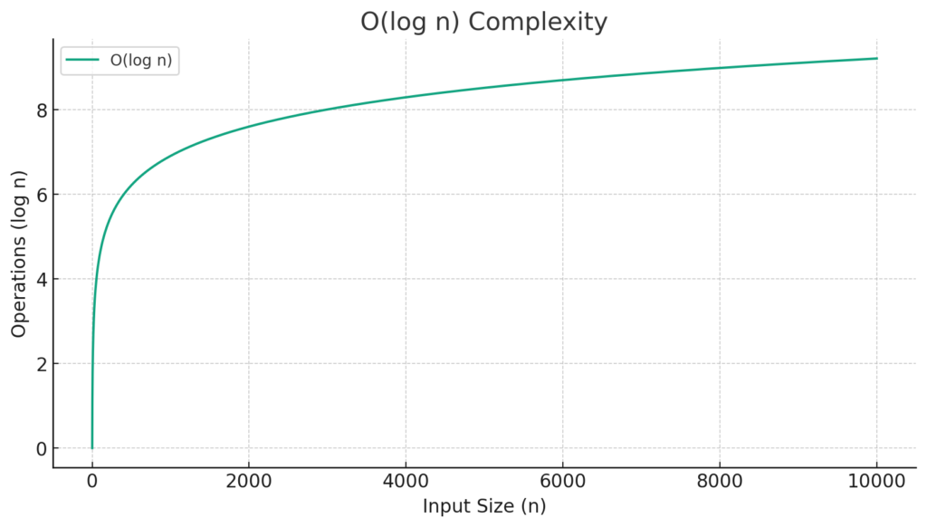
The graph below visualizes the O(log n) complexity. As shown, as the input size (n) increases, the number of operations (log n) increases at a logarithmic rate, which is much slower than linear, demonstrating the efficiency of algorithms with logarithmic time complexity.
import matplotlib.pyplot as plt
import numpy as np

# Generate a range of values from 1 to 10000
x = np.arange(1, 10001, 1)
# Calculate O(log n) complexity
y = np.log(x)

plt.figure(figsize=(10, 5))
plt.plot(x, y, label='O(log n)')
plt.title('O(log n) Complexity')
plt.xlabel('Input Size (n)')
plt.ylabel('Operations (log n)')
plt.legend()
plt.grid(True)
plt.show()

The Future of O(log n) in Computer Science Education
As we progress through the digital age, understanding the implications of algorithmic efficiency becomes increasingly important. O(log n) is not just a concept to be memorized; it’s a principle that will be encountered repeatedly, underscoring the importance of efficient algorithm design.


